9 Documenting your results with R Markdown
9.1 Intro
Another benefit with using R is the ability to pair your statistical analysis with a method of easily documenting the results from it. With R Markdown, you can easily create a document which combines your code, the results from your code, as well as any text or outside images that accompany the analysis. This tutorial details how to use R Markdown; in fact, all of these tutorials were created using it. Thus, you can also supplement the information in this tutorial by studying the included R Markdown files which created all of the other tutorials.
9.2 Starting Your R Markdown
To create a new R Markdown file, in R Studio select File>New File>R Markdown… . Then, you will see a window pop-up titled “New R Markdown”. Here, you specify the type of file you wish to create. The standard type is a document (HTML, PDF, or Word) but you have some other options such as creating a slide show (Presentation). In these tutorials, we just cover documents. Within the Document type, you must select what file type you would like. Since it does not have traditional “page” separators like PDF and Word do, HTML is generally recommended and will be covered in these tutorials. You can also choose a title and author for your document using their respective fields. Finally, select Ok to create your new R Markdown file. You will see it appear as a tab in your R Studio session, similar to when a new script is created.
9.3 Understanding the R Markdown editor
When creating a new HTML-type R Markdown document, you should see the following window in your R Studio session:
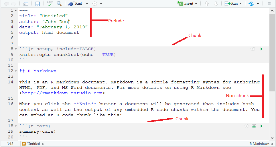
which looks similar to a script. Here is where you edit and create the content of your R Markdown. A R Markdown has three main components: the Prelude, the Chunk, and the Non-chunk, which are labeled in the above document for reference.
9.3.1 Prelude
In the Prelude, you specify settings and headers for your R Markdown. Some headers you can specify include the title, author, and date. The main setting you may alter is the output setting, which determines which file types are used when creating your document. You can specify multiple file types, or leave it as the single type you chose when creating your Markdown (HTML in the above example). For example, to add a PDF type as an output, add in pdf_document: default below output::.
9.3.2 Chunk
A chunk is a specially marked part of your Markdown document where you place R code to have run. You will generally have multiple chunks throughout your Markdown which represent specific components of your analysis. When you create your Markdown file and turn it into a document, these chunks are run in order and any output from them is shown in the document, in the order that their respective chunk appears. A chunk is marked using {r name} to start, as in the following example:

You can see that the chunk is shaded in gray and adds in a few icons on the upper right of this shaded space. A chunk has a few components. First, you must name your chunk, which allows you to easily refer to what the code in the chunk does and to facilitate the organization of your document. In the above example, “name” was used as the chunk’s name. Note that each chunk must have a different name or else you will receieve an error when the R Markdown file is compiled. You can also specify a number of options for your chunk inside {r …}, where each option is placed in … and separated by a comma. These options are specified just like arguments in a R function. Note that the chunk’s name is technically an option, so you must separate it from the other options using a comma. Some common options include:
- echo=TRUE or FALSE
If TRUE is selected, the actual code in the chunk appears in your document along with the results it produced. If FALSE is selected, the code does not appear and only the output does
- warning=TRUE or FALSE
If TRUE is selected (is by default), all outputted warnings from the code are included in the document. If FALSE is selected, these wanrings are not included.
- include=TRUE or FALSE
If TRUE is selected (is by default), the output from the code is included in the document. If FALSE is selected, the code is still run but the output is not included in the document. This can be useful if you use certain calculations from this chunk in later chunks and the actual output from this chunk is not of interest.
Some others include eval= and messages=; see online for more details and more options that you can set. Inside this shaded space is where you place your code for that part of the analysis. This works exactly like how writing a script works; you are simply writing the usual R code. Finally, let us discuss the icons on the upper right side. The left-most option can be avoided as it simply lets you alter the settings of the chunk instead of using the options through {r }. The next option has R run all of the chunks above this chunk, which may be necessary when this chunk’s code depends on the chunks above it. The last option runs only the current chunk, which is necessary to view the output of the chunk and/or verify the code within it is operating correctly as you create your R Markdown document. Note that when you run a chunk, its output will be shown right below it. To obtain everything that the code in the chunk produces (output, warnings, errors, etc.), make sure to select the Console tab in the lower-left hand window, which contains the usual R console. We will discuss the R Markdown tab later. Note that to specify options for all chunks in your R Markdown (i.e., “global options”), include the following command in a separate chunk at the top of the document (but below the Prelude):
knitr::opts_chunk$set(…)
where the options of interest are placed as argument separated by commas. You can override these global options for specific chunks but setting the override in the chunk(s) of interest as discussed above. See the .RMD files which created these tutorials for further detail.
9.3.3 Non-chunk
The white space outside of your Prelude is where you place the non-R code components of your document. This space largely works like a Word document; you can place text, images, tables, etc. inside of it. This combination of R code, its results, and the Word document-like capabilities is what allows you to create a comprehensive report for your analysis within a single file. You can also format the text which appears in this space. Surrounding your text with ** ** bolds the text, and with * * italicizes the text. To add a subscript, use _ and to add a superscript use ^ . To mark a webpage link, use /linked phrase where “linked phrase” is the text that appears in the document and () holds the actual URL. Note that when adding in links to webpages, if you are creating a document in HTML format, you will have to add self_contained: no to your Prelude below html_document: default. To add images, use !optional caption text where [] specifies the image caption (which can be empty) and () holds the file name for the image. If the image is in the same folder as the Markdown file, you can just include the file name. Otherwise, you must provide the whole file path (or use relative path names if you are familar with them).
Along with usual text, you can also specify headers within this space. To start a header, use # and type your header text next to it. Using ## creates a sub header, ### creates a sub-sub header, etc. Note that these headers must be on their own lines in your R Markdown file to be recognized as headers and not just the #, ##, etc. characters. See the R Markdown Cheatsheet for more capabilities as well as for a review of what was discussed above.
9.4 Creating your document from the R Markdown file
When you have finished creating your R Markdown file, you can now “compile” it to create the final document. You can think of your R Markdown file as the “instructions” the software uses to create the final document, just like scripts are the “instructions” R uses to complete your analysis. Thus, these R Markdown files are essentially more complex scripts and are denoted by the file type .Rmd instead of .R .
With your R Markdown file open in R studio, you create the corresponding document using the Knit button at the top. This will compile your R Markdown into the document file types that you specified in the Prelude. You will see the progress of the compilation as well as any errors or other messages created during the compilation process in the lower left-hand window of R Studio, in the R Markdown tab.
9.5 Creating tables with R Markdown
One of the most useful features of R Markdown is the ability to create publication-quality tables. When combined with the plots from ggplot2, this enables you to create detailed reports in R Markdown that display all of your results in a publication-quality format. Recall from our past tutorials that when you output tables with your R script, the format is crude looking.
library(stats)
aosi_data <- read.csv("Data/cross-sec_aosi.csv", stringsAsFactors=FALSE, na.strings = ".")
table_ex_xtabs <- xtabs(~Gender+Study_Site, data=aosi_data)
table_ex_xtabs
## Study_Site
## Gender PHI SEA STL UNC
## Female 55 67 60 53
## Male 94 85 85 88In this section, we will detail how to create custom tables to summarize a variety of standard analyses, as well as how to output them in a visually pleasing format using kable().
9.5.1 Summary statistics
First, we discuss some functions which create publication quality summary statistics tables. We have discussed previously how to create some crude-looking summary statistics tables in R (see Chapter 7), however here we discuss some functions which take advantage of R Markdown to better display these results. The first function we discuss is the function describe() from the Hmisc package, which was discussed in Chapter 7. When used in R Markdown, the results look the same as when used in a usual R script.
## aosi_data
##
##  8  Variables      587  Observations
## ---------------------------------------------------------------------------
## Identifiers
##        n  missing distinct     Info     Mean      Gmd      .05      .10
##      587        0      587        1      294      196     30.3     59.6
##      .25      .50      .75      .90      .95
##    147.5    294.0    440.5    528.4    557.7
##
## lowest :   1   2   3   4   5, highest: 583 584 585 586 587
## ---------------------------------------------------------------------------
## GROUP
##        n  missing distinct
##      587        0        4
##
## Value      HR_ASD HR_neg LR_ASD LR_neg
## Frequency      95    318      3    171
## Proportion  0.162  0.542  0.005  0.291
## ---------------------------------------------------------------------------
## Study_Site
##        n  missing distinct
##      587        0        4
##
## Value        PHI   SEA   STL   UNC
## Frequency    149   152   145   141
## Proportion 0.254 0.259 0.247 0.240
## ---------------------------------------------------------------------------
## Gender
##        n  missing distinct
##      587        0        2
##
## Value      Female   Male
## Frequency     235    352
## Proportion    0.4    0.6
## ---------------------------------------------------------------------------
## V06.aosi.Candidate_Age
##        n  missing distinct     Info     Mean      Gmd      .05      .10
##      482      105       38    0.996    6.595   0.7179    5.800    6.000
##      .25      .50      .75      .90      .95
##    6.100    6.400    6.900    7.500    8.095
##
## lowest : 5.1 5.5 5.6 5.7 5.8, highest: 8.7 8.9 9.0 9.3 9.4
## ---------------------------------------------------------------------------
## V06.aosi.total_score_1_18
##        n  missing distinct     Info     Mean      Gmd      .05      .10
##      482      105       24    0.994    9.562    4.622        4        5
##      .25      .50      .75      .90      .95
##        7        9       12       15       17
##
## lowest :  1  2  3  4  5, highest: 20 21 22 24 28
## ---------------------------------------------------------------------------
## V12.aosi.Candidate_Age
##        n  missing distinct     Info     Mean      Gmd      .05      .10
##      512       75       37    0.994    12.59   0.7036     11.9     12.0
##      .25      .50      .75      .90      .95
##     12.2     12.5     12.9     13.4     13.9
##
## lowest :  0.0 11.4 11.6 11.7 11.8, highest: 14.9 15.1 15.6 15.9 16.7
## ---------------------------------------------------------------------------
## V12.aosi.total_score_1_18
##        n  missing distinct     Info     Mean      Gmd      .05      .10
##      512       75       20     0.99     4.98    3.901        1        1
##      .25      .50      .75      .90      .95
##        2        4        7       10       12
##
## Value          0     1     2     3     4     5     6     7     8     9
## Frequency     23    51    66    68    72    51    34    40    27    18
## Proportion 0.045 0.100 0.129 0.133 0.141 0.100 0.066 0.078 0.053 0.035
##
## Value         10    11    12    13    14    15    16    17    20    22
## Frequency     21    10     8     7     6     4     3     1     1     1
## Proportion 0.041 0.020 0.016 0.014 0.012 0.008 0.006 0.002 0.002 0.002
## ---------------------------------------------------------------------------
However, we can force the output to be of HTML format to match with our HTML formatted R Markdown document using the function html() which is also in the Hmisc package. This greatly improves the look of the output. We combine it with the pipe operator (see Chapter 4) to make the code more efficient. This html() function can be used for most output to force it to HTML form when you compile your R Markdown file into an HTML document.
8 Variables 587 Observations
Identifiers

| n | missing | distinct | Info | Mean | Gmd | .05 | .10 | .25 | .50 | .75 | .90 | .95 |
|---|---|---|---|---|---|---|---|---|---|---|---|---|
| 587 | 0 | 587 | 1 | 294 | 196 | 30.3 | 59.6 | 147.5 | 294.0 | 440.5 | 528.4 | 557.7 |
GROUP

| n | missing | distinct |
|---|---|---|
| 587 | 0 | 4 |
 Value      HR_ASD HR_neg LR_ASD LR_neg
 Frequency      95    318      3    171
 Proportion  0.162  0.542  0.005  0.291
Study_Site

| n | missing | distinct |
|---|---|---|
| 587 | 0 | 4 |
 Value        PHI   SEA   STL   UNC
 Frequency    149   152   145   141
 Proportion 0.254 0.259 0.247 0.240
Gender
| n | missing | distinct |
|---|---|---|
| 587 | 0 | 2 |
 Value      Female   Male
 Frequency     235    352
 Proportion    0.4    0.6
V06.aosi.Candidate_Age

| n | missing | distinct | Info | Mean | Gmd | .05 | .10 | .25 | .50 | .75 | .90 | .95 |
|---|---|---|---|---|---|---|---|---|---|---|---|---|
| 482 | 105 | 38 | 0.996 | 6.595 | 0.7179 | 5.800 | 6.000 | 6.100 | 6.400 | 6.900 | 7.500 | 8.095 |
V06.aosi.total_score_1_18

| n | missing | distinct | Info | Mean | Gmd | .05 | .10 | .25 | .50 | .75 | .90 | .95 |
|---|---|---|---|---|---|---|---|---|---|---|---|---|
| 482 | 105 | 24 | 0.994 | 9.562 | 4.622 | 4 | 5 | 7 | 9 | 12 | 15 | 17 |
V12.aosi.Candidate_Age

| n | missing | distinct | Info | Mean | Gmd | .05 | .10 | .25 | .50 | .75 | .90 | .95 |
|---|---|---|---|---|---|---|---|---|---|---|---|---|
| 512 | 75 | 37 | 0.994 | 12.59 | 0.7036 | 11.9 | 12.0 | 12.2 | 12.5 | 12.9 | 13.4 | 13.9 |
V12.aosi.total_score_1_18

| n | missing | distinct | Info | Mean | Gmd | .05 | .10 | .25 | .50 | .75 | .90 | .95 |
|---|---|---|---|---|---|---|---|---|---|---|---|---|
| 512 | 75 | 20 | 0.99 | 4.98 | 3.901 | 1 | 1 | 2 | 4 | 7 | 10 | 12 |
 Value          0     1     2     3     4     5     6     7     8     9    10    11
 Frequency     23    51    66    68    72    51    34    40    27    18    21    10
 Proportion 0.045 0.100 0.129 0.133 0.141 0.100 0.066 0.078 0.053 0.035 0.041 0.020

 Value         12    13    14    15    16    17    20    22
 Frequency      8     7     6     4     3     1     1     1
 Proportion 0.016 0.014 0.012 0.008 0.006 0.002 0.002 0.002
9.5.2 General tables
In R Markdown, you can essentially create and format any table you can think of by simply creating a matrix object containing the table of interest and then applying a special function to format it into HTML form. Two of these “special” functions are kable() from the kableExtra package and htmlTable() from the htmlTable package. We cover kable() here though curious readers can also learn about htmlTable() online.
First, we need to create a matrix which contains the results of interest in the row by column formt that matches the format of our desired table.
For example, suppose we wanted to conduct an ANOVA analysis with some of the Mullen composite standard score and ASO total score with respect to diagnosis group (High Risk: ASD, High Risk: Negative, and Low Risk: Negative).
library(lsmeans)

data <- read.csv("Data/Cross-sec_full.csv", stringsAsFactors=FALSE, na.strings = c(".", "", " "))

data_v2 <- data %>%
  mutate(GROUP=fct_recode(GROUP, "HR: Negative"="HR_neg", "LR: Negative"="LR_neg",
                          "HR: ASD"="HR_ASD"))

## Mullen
# Get means and CIs
composite_anova <- lm(V12.mullen.composite_standard_score~GROUP, data=data_v2)
composite_for_table <- as.data.frame(lsmeans(composite_anova, specs="GROUP"))
composite_for_table <- composite_for_table %>%
  mutate(Mean_SE=paste(round(lsmean,2),
                       paste("(",round(SE,2),")",sep=""),sep=" "))  %>%
  select(GROUP, Mean_SE)
composite_for_table <- t(composite_for_table)
colnames(composite_for_table) <- composite_for_table[1,]
composite_for_table <- composite_for_table[-1,]
composite_for_table <- c("Score"="Mullen Composite", composite_for_table)

## AOSI
# Get means and CIs
aosi_anova <- lm(V12.aosi.total_score_1_18~GROUP, data=data_v2)
aosi_for_table <- as.data.frame(lsmeans(aosi_anova, specs="GROUP"))
aosi_for_table <- aosi_for_table %>%
  mutate(Mean_SE=paste(round(lsmean,2),
                       paste("(",round(SE,2),")",sep=""),sep=" ")) %>%
  select(GROUP, Mean_SE)
aosi_for_table <- t(aosi_for_table)
colnames(aosi_for_table) <- aosi_for_table[1,]
aosi_for_table <- aosi_for_table[-1,]
aosi_for_table <- c("Score"="AOSI Total", aosi_for_table)

## Calculate overall F tests for each score
composite_f_stat <- round(anova(composite_anova)$`F value`[1],2)
aosi_f_stat <- round(anova(aosi_anova)$`F value`[1],2)

composite_f_test <- ifelse(anova(composite_anova)$`Pr(>F)`[1]>0.001,                         round(anova(composite_anova)$`Pr(>F)`[1],3),"<0.001")
aosi_f_test <- ifelse(anova(aosi_anova)$`Pr(>F)`[1]>0.001,
                          round(anova(aosi_anova)$`Pr(>F)`[1],3),"<0.001")

## Combine into single table
anova_table <- rbind(composite_for_table, aosi_for_table)
anova_table <- cbind(anova_table,
                     "F Statistic"=c(composite_f_stat,
                                     aosi_f_stat),
                     "P-value"=c(composite_f_test, aosi_f_test))

# Remove rownames, can see they are not needed (composite_for_table, etc.)
rownames(anova_table) <- NULL # (NULL => empty, different from missing NA)

# Print out table in crude format (default format from R output)
anova_table
## Score HR: ASD HR: Negative LR_ASD
## [1,] "Mullen Composite" "92.48 (1.44)" "101.21 (0.76)" "100.67 (7.47)"
## [2,] "AOSI Total" "7.34 (0.39)" "4.84 (0.21)" "3.67 (2)"
## LR: Negative F Statistic P-value
## [1,] "105.77 (1.05)" "18.57" "<0.001"
## [2,] "3.99 (0.29)" "16.68" "<0.001"Let us go over the above code used to produce the table of interest. First, for each score, we
Ran an ANOVA with the domain score as the outcome and diagnosis groups as the groups for comparison. We saved the ANOVA results as an object.
Then, we calculated the least square means for each group from the ANOVA results. We saved these means as a data frame to make the output easier to manipulate. Using mutate(), we created a new column called Mean_SE which combined the mean and mean’s standard error (SE) together into the usual “mean (SE)” format. We did this use the function paste(). This function allows you to combine values x, y, and z into a single string (for example) using paste(x, y, z, sep=“w”) where sep=“w” denotes the string used to separate each input. For example, sep=“,” would result in “x,y,z”. We also rounded these means and SEs to 2 decimal places using the function round(). We then added a column called “Domain” which contains the name of the Mullen domain used in the ANOVA model.
We then combined all of these estimated means and SEs across the domains using rbind().
We calculated the F test statistics and p-values for each of these ANOVA analyses. We added these as columns to the final table (notice the use of c() to combine all of the domain F statistics and p-values into two separate columns).
While it took some code to do, we now have a table which is structured as we had desired for the ANOVA results. You can create similar tables for regression analyses by using the above code and making some changes to reflect the use of lm() or lme() instead of aov(). This pasting together of various results using cbind() and rbind(), as well as editing the results using paste(), round(), and the functions from dplyr is a general method you can use to create your tables for any analysis.
Finally, we use kable() from the kableExtra package to print out this table in HTML format. The first argument is the table/matrix/data frame of interest. Some other useful arguments include row.names= which lets you specify that names of the rows of the output, col.names= which does the same for the column names, and caption= which allows you to specify the title for the output. Here, we omit the row names and just have the column names be the column names of the actual R object. To adjust more aspects, use the function kable_styling(); see the documentation for this function to learn more. This function also changes the overall look of the output and it is recommended to always apply it, even if you do not use any of its arguments (see below).
library(kableExtra)

kable(anova_table,
      col.names = colnames(anova_table),
      caption="Comparison of group means from regression of Mullen composite and AOSI total score on diagnosis group.  Estimated group means and their corresponding standard errors (SE), rounded to two decimal spaces, are provided for each score  These comparisons were done for Expressive Language, Fine Motor, and Gross Motor at 12 months.  For each of these, the p-value and test statistic corresponding to the ANOVA F-test for group differences is reported.") %>%
kable_styling()| Score | HR: ASD | HR: Negative | LR_ASD | LR: Negative | F Statistic | P-value |
|---|---|---|---|---|---|---|
| Mullen Composite | 92.48 (1.44) | 101.21 (0.76) | 100.67 (7.47) | 105.77 (1.05) | 18.57 | <0.001 |
| AOSI Total | 7.34 (0.39) | 4.84 (0.21) | 3.67 (2) | 3.99 (0.29) | 16.68 | <0.001 |
For more details on using kable() and kableExtra(), as well as additional examples, please see the following.
9.6 Practice with R Markdown
For examples of R Markdown files and the corresponding documents that they create, please view the R Markdown files that created all of these HTML-type R tutorials. Reading through these R Markdown files and compiling them using Knit will be the best way of understand the capabilities of R Markdown, as well as how to use them.